output_dir <- "output"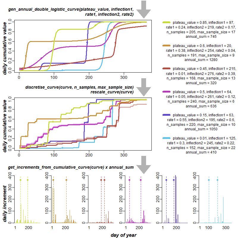
plot_file_format <- c("png", "eps")[1] # modify index number to change format5 Demonstration of parameter variation: precipitation
Choose file format for generated figures:
Load source file containing the R implementation of the Weather model:
source("source/weatherModel.R")Set up six variations of parameter settings for the annual double logistic curve, discretisation, and annual precipitation, assuming a year length of 365 days. The random generator SEED used in discretisation is fixed:
SEED <- 0
YEAR_LENGTH <- 365

# Function to create parameter matrix
create_param_matrix <- function(x, ncol, nrow) {
  matrix(x, ncol = ncol, nrow = nrow, byrow = TRUE)
}

# Double logistic curve parameters
par_values_double_logistic <- create_param_matrix(c(
  0.01, 125, 0.3,  245, 0.22,
  0.15, 63,  0.55, 195, 0.6,
  0.5,  64,  0.05, 261, 0.12,
  0.45, 215, 0.01, 276, 0.39,
  0.6,  20,  0.38, 254, 0.04,
  0.85, 97,  0.24, 219, 0.17
  ), ncol = 5, nrow = 6
)
colnames(par_values_double_logistic) <- c("plateau_value", "inflection1", "rate1", "inflection2", "rate2")

# Discretisation parameters
par_values_discretisation <- create_param_matrix(c(
  152, 22,
  220, 10,
  240, 6,
  168, 13,
  191, 9,
  205, 17
  ), ncol = 2, nrow = 6
)
colnames(par_values_discretisation) <- c("n_samples", "max_sample_size")

annual_sum_values <- c(410, 1050, 636, 320, 1280, 745)

num_runs <- nrow(par_values_double_logistic)
Create a colour palette for plotting:
num_cold_colours <- num_runs %/% 2
num_warm_colours <- num_runs - num_cold_colours

create_color_sequence <- function(start, end, n) {
  seq(start, end, length.out = n)
}

create_color_values <- function(h_range, s_range, v_range, n) {
  cbind(
    h = create_color_sequence(h_range[1], h_range[2], n) / 360,
    s = create_color_sequence(s_range[1], s_range[2], n) / 100,
    v = create_color_sequence(v_range[1], v_range[2], n) / 100
  )
}

color_palette_values <- rbind(
  create_color_values(c(198.6, 299.4), c(61.6, 75.3), c(95.2, 76.4), num_cold_colours),
  create_color_values(c(5.15, 67.5), c(67, 77.8), c(73.7, 86.4), num_warm_colours)
)

color_palette <- apply(color_palette_values, 1, function(x) hsv(x[1], x[2], x[3]))
Plot curves:
# Helper functions
create_data_frame <- function(rows, cols) {
  data.frame(matrix(0, nrow = rows, ncol = cols))
}

create_plot <- function(x_range, y_range, ...) {
  plot(x_range, y_range, type = "n", xlab = "", ylab = "", ...)
}

add_text <- function(x, y, label, ...) {
  text(x = x, y = y, labels = label, ...)
}

draw_curve <- function(curve, color, ...) {
  lines(1:length(curve), curve, col = color, ...)
}

draw_points <- function(x, y, color, ...) {
  points(x, y, col = color, ...)
}

# Main plotting function
plot_annual_double_logistic <- function(par_values_double_logistic, par_values_discretisation, annual_sum_values) {

  # Create data frames
  double_logistic_curves <- create_data_frame(YEAR_LENGTH, num_runs)
  discretised_double_logistic_curves <- create_data_frame(YEAR_LENGTH, num_runs)
  daily_precipitation <- create_data_frame(YEAR_LENGTH, num_runs)

  # Layout setup
  layout_matrix <- matrix(c(14, 14, 14, 14, 14, 17, 17,
                            1,   5,  5,  5,  5, 17, 17,
                            15, 15, 15, 15, 15, 17, 17,
                            2,   6,  6,  6,  6, 17, 17,
                            16, 16, 16, 16, 16, 17, 17,
                            3,   7,  8,  9, 10, 11, 12,
                            4,  13, 13, 13, 13, 13, 13),
                          nrow = 7, ncol = 7, byrow = TRUE)
  layout(layout_matrix,
         widths = c(2.5, rep(10, 5), 12),
         heights = c(4, 12, 4, 12, 4, 12, 1))

  par(mgp = c(3, 0.4, 0), tcl = -0.4, cex = graphic_scale * 1.2, cex.axis = graphic_scale * (font_rescale + axis_text_rescale))

  # Y-axis titles
  y_axis_titles <- c("daily cumulative value", "daily cumulative value", "daily increment")
  for (i in 1:3) {
    par(mar = c(0, 0, 0, 0))
    create_plot(c(0, 1), c(0, 1), ann = FALSE, bty = 'n', xaxt = 'n', yaxt = 'n')
    add_text(0.5, 0.5, y_axis_titles[i], font = 4,
             cex = graphic_scale * (0.7 + font_rescale + margin_text_rescale), srt = 90)
  }

  # Empty plot
  create_plot(c(0, 1), c(0, 1), ann = FALSE, bty = 'n', xaxt = 'n', yaxt = 'n')

  # Double logistic curves plot
  par(mar = c(1, 1, 0.1, 1), cex.axis = graphic_scale * (font_rescale + axis_text_rescale))
  create_plot(c(1, YEAR_LENGTH), c(0, 1))

  for (i in 1:nrow(par_values_double_logistic)) {
    curve <- gen_annual_double_logistic_curve(
      plateau_value = par_values_double_logistic[i, 1],
      inflection1 = par_values_double_logistic[i, 2],
      rate1 = par_values_double_logistic[i, 3],
      inflection2 = par_values_double_logistic[i, 4],
      rate2 = par_values_double_logistic[i, 5],
      year_length = YEAR_LENGTH)

    draw_curve(curve, color_palette[i], lwd = graphic_scale * 3)
    draw_points(c(par_values_double_logistic[i, 2], par_values_double_logistic[i, 4]),
                c(curve[par_values_double_logistic[i, 2]], curve[par_values_double_logistic[i, 4]]),
                color_palette[i], pch = 19)

    double_logistic_curves[,i] <- curve
  }

  # Discretised double logistic plot
  create_plot(c(1, YEAR_LENGTH), c(0, 1))

  for (i in 1:nrow(par_values_double_logistic)) {
    curve <- discretise_curve(
      curve = double_logistic_curves[,i],
      n_samples = par_values_discretisation[i, 1],
      max_sample_size = par_values_discretisation[i, 2],
      seed = SEED)

    draw_curve(curve, adjustcolor(color_palette[i], alpha.f = 0.5), lwd = graphic_scale * 3)
    draw_points(c(par_values_double_logistic[i, 2], par_values_double_logistic[i, 4]),
                c(curve[par_values_double_logistic[i, 2]], curve[par_values_double_logistic[i, 4]]),
                adjustcolor(color_palette[i], alpha.f = 0.5), pch = 19)

    curve <- rescale_curve(curve)

    draw_curve(curve, color_palette[i], lwd = graphic_scale * 3)
    draw_points(c(par_values_double_logistic[i, 2], par_values_double_logistic[i, 4]),
                c(curve[par_values_double_logistic[i, 2]], curve[par_values_double_logistic[i, 4]]),
                color_palette[i], pch = 19)

    discretised_double_logistic_curves[,i] <- curve
  }

  # Daily precipitation plots
  par(mar = c(2, 1, 0.1, 1), cex.axis = graphic_scale * (font_rescale + axis_text_rescale))

  daily_precipitation <- sapply(1:nrow(par_values_double_logistic), function(i) {
    get_increments_from_cumulative_curve(discretised_double_logistic_curves[,i]) * annual_sum_values[i]
  })

  maxdaily_precipitation <- max(daily_precipitation)

  for (i in nrow(par_values_double_logistic):1) {
    barplot(daily_precipitation[,i],
            names.arg = c("1", rep(NA, 98), "100", rep(NA, 99), "200", rep(NA, 99), "300", rep(NA, 65)),
            ylim = c(0, maxdaily_precipitation),
            col = color_palette[i],
            border = color_palette[i])

    draw_points(c(par_values_double_logistic[i, 2], par_values_double_logistic[i, 4]),
                rep(maxdaily_precipitation * 0.9, 2),
                color_palette[i], pch = 19)

    abline(v = par_values_double_logistic[i, 2], col = color_palette[i], lty = 2)
    abline(v = par_values_double_logistic[i, 4], col = color_palette[i], lty = 2)
  }

  # X-axis title
  par(mar = c(0, 0, 0, 0))
  create_plot(c(0, 1), c(0, 1), ann = FALSE, bty = 'n', xaxt = 'n', yaxt = 'n')
  add_text(0.5, 0.6, "day of year", font = 4,,
           cex = graphic_scale * (0.7 + font_rescale + margin_text_rescale))

  # Infographic bits
  draw_infographic <- function(label) {
    create_plot(c(0, 1), c(0, 1), ann = FALSE, bty = 'n', xaxt = 'n', yaxt = 'n')
    polygon(x = arrow_pos_x[1] + (arrow_pos_x[2] - arrow_pos_x[1]) * arrow_points_x,
            y = arrow_points_y,
            col = rgb(0,0,0, alpha = 0.3),
            border = NA)
    add_text(text_pos[1], text_pos[2],
             label, font = 4, cex = graphic_scale * (0.65 + font_rescale + infographic_text_rescale), adj = c(1, 0.5))
  }

  arrow_points_x <- c(1/3, 2/3, 2/3, 1, 0.5, 0, 1/3, 1/3)
  arrow_points_y <- c(1, 1, 0.5, 0.5, 0, 0.5, 0.5, 1)
  arrow_pos_x <- c(0.9, 1)
  text_pos <- c(0.88, 0.4)

  par(mar = c(0, 0, 0, 0))

  infographic_labels <- c(
    "gen_annual_double_logistic_curve(plateau_value, inflection1,\nrate1, inflection2, rate2)",
    "discretise_curve(curve, n_samples, max_sample_size)\nrescale_curve(curve)",
    "get_increments_from_cumulative_curve(curve) x annual_sum"
  )

  lapply(infographic_labels, draw_infographic)

  # Legend
  par(mar = c(0, 0, 0, 0))
  create_plot(c(0, 1), c(0, nrow(par_values_double_logistic) + 1),
              ann = FALSE, bty = 'n', xaxt = 'n', yaxt = 'n')

  y_pos <- c(0.5, seq(0.1, -0.3, length.out = 3))
  x_pos <- 0.55
  jump <- 1

  for (i in 1:nrow(par_values_double_logistic)) {
    legend(x = 0,
           y = (y_pos[1] + jump * i),
           legend = substitute(
             paste("plateau_value = ", plateau_value, ", ",
                   "inflection1 = ", inflection1, ", "),
             list(plateau_value = par_values_double_logistic[i, 1],
                  inflection1 = par_values_double_logistic[i, 2])),
           col = color_palette[i],
           lwd = graphic_scale * 6, cex = graphic_scale * (font_rescale + legend_text_rescale),
           title = NULL,
           bty = "n")
    add_text(x_pos,
             (y_pos[2] + jump * i),
             substitute(
               paste("rate1 = ", rate1, ", ",
                     "inflection2 = ", inflection2, ", ",
                     "rate2 = ", rate2, ","),
               list(rate1 = par_values_double_logistic[i, 3],
                    inflection2 = par_values_double_logistic[i, 4],
                    rate2 = par_values_double_logistic[i, 5])),
             cex = graphic_scale * (font_rescale + legend_text_rescale))
    add_text(x_pos,
             (y_pos[3] + jump * i),
             substitute(
               paste("n_samples = ", n_samples, ", ",
                     "max_sample_size = ", max_sample_size),
               list(n_samples = par_values_discretisation[i, 1],
                    max_sample_size = par_values_discretisation[i, 2])),
             cex = graphic_scale * (font_rescale + legend_text_rescale))
    add_text(x_pos,
             (y_pos[4] + jump * i),
             substitute(
               paste("annual_sum = ", annual_sum),
               list(annual_sum = annual_sum_values[i])),
             cex = graphic_scale * (font_rescale + legend_text_rescale))
  }
}

# Main execution
plot_name <- file.path(output_dir, paste0("Fig5-annualDoubleLogisticCurve.", plot_file_format))

if (plot_file_format == "png") {
  graphic_scale <- 1
  font_rescale <- 1.2
  axis_text_rescale <- -0.25
  margin_text_rescale <- -0.7
  infographic_text_rescale <- -0.9
  legend_text_rescale <- -0.35
  png(plot_name, width = graphic_scale * 800, height = graphic_scale * 800)
} else if (plot_file_format == "eps") {
  graphic_scale <- 1.2
  font_rescale <- 0.1
  axis_text_rescale <- 1
  margin_text_rescale <- 0
  infographic_text_rescale <- 0
  legend_text_rescale <- 0.5
  extrafont::loadfonts(device = "postscript")
  grDevices::cairo_ps(filename = plot_name, pointsize = 12,
                      width = graphic_scale * 10, height = graphic_scale * 10,
                      onefile = FALSE, family = "sans")
}
plot_annual_double_logistic(par_values_double_logistic, par_values_discretisation, annual_sum_values)
dev.off()
svg
2 knitr::include_graphics(plot_name)