output_dir <- "output"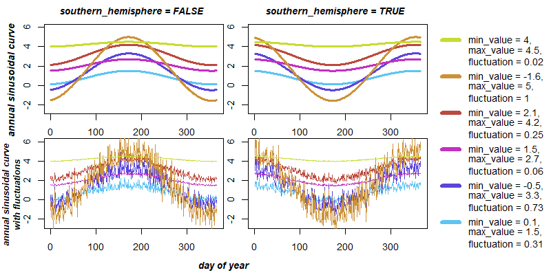
plot_file_format <- c("png", "eps")[1] # modify index number to change format4 Demonstration of parameter variation: solar radiation and temperature
Choose file format for generated figures:
Load source file containing the R implementation of the Weather model:
source("source/weatherModel.R")Set up six variations of parameter settings (i.e. min_value, max_value, is_south_hemisphere), assuming length of year of 365 days:
SEED <- 0
YEAR_LENGTH <- 365
is_southern_hemisphere_values <- c(FALSE, TRUE)

par_values_annual_sinusoid <- matrix(
  c(0.1, 1.5, 0.31,
    -0.5, 3.3, 0.73,
    1.5, 2.7, 0.06,
    2.1, 4.2, 0.25,
    -1.6, 5, 1,
    4, 4.5, 0.02),
  ncol = 3, byrow = TRUE
)

min_min_value <- min(par_values_annual_sinusoid[,1] - par_values_annual_sinusoid[,3])
max_max_value <- max(par_values_annual_sinusoid[,2] + par_values_annual_sinusoid[,3])

num_runs <- nrow(par_values_annual_sinusoid)
Create a colour palette for plotting:
num_cold_colours <- num_runs %/% 2
num_warm_colours <- num_runs - num_cold_colours

create_color_sequence <- function(start, end, n) {
  seq(start, end, length.out = n)
}

create_color_values <- function(h_range, s_range, v_range, n) {
  cbind(
    h = create_color_sequence(h_range[1], h_range[2], n) / 360,
    s = create_color_sequence(s_range[1], s_range[2], n) / 100,
    v = create_color_sequence(v_range[1], v_range[2], n) / 100
  )
}

color_palette_values <- rbind(
  create_color_values(c(198.6, 299.4), c(61.6, 75.3), c(95.2, 76.4), num_cold_colours),
  create_color_values(c(5.15, 67.5), c(67, 77.8), c(73.7, 86.4), num_warm_colours)
)

color_palette <- apply(color_palette_values, 1, function(x) hsv(x[1], x[2], x[3]))
Plot curves:
# Helper functions
plot_empty <- function() {
  plot(c(0, 1), c(0, 1), ann = FALSE, bty = 'n', type = 'n', xaxt = 'n', yaxt = 'n')
}

add_text <- function(x, y, label, cex_factor = 0.6, srt = 0) {
  text(x = x, y = y, labels = label, font = 4,
       cex = graphic_scale * (cex_factor + font_rescale + margin_text_rescale), srt = srt)
}

# Main plotting function
plot_annual_sinusoid <- function(par_values_annual_sinusoid, is_southern_hemisphere_values, min_min_value, max_max_value) {
  layout(matrix(c(1,  2,  3, 12,
                  4,  5,  6, 12,
                  7,  8,  9, 12,
                  10, 11, 11, 12),
                nrow = 4, ncol = 4, byrow = TRUE),
         widths = c(1, 10, 10, 6),
         heights = c(2, 10, 10, 2))

  par(cex = graphic_scale * 1.2, mar = c(0, 0, 0, 0))

  # Titles
  plot_empty()
  for (hemisphere in c("FALSE", "TRUE")) {
    plot_empty()
    add_text(0.55, 0.5, paste("southern_hemisphere =", hemisphere))
  }

  # Y-axis titles and plots
  plot_empty()
  add_text(0.5, 0.5, "annual sinusoidal curve", srt = 90)

  par(mar = c(2, 2, 0.1, 0.1))

  for (is_southern_hemisphere in is_southern_hemisphere_values) {
    plot(c(1, YEAR_LENGTH), c(min_min_value, max_max_value), type = "n", xlab = "", ylab = "")

    for (i in 1:nrow(par_values_annual_sinusoid)) {
      curve <- gen_annual_sinusoid(
        min_value = par_values_annual_sinusoid[i, 1],
        max_value = par_values_annual_sinusoid[i, 2],
        year_length = YEAR_LENGTH,
        is_southern_hemisphere = is_southern_hemisphere)

      lines(1:length(curve), curve, col = color_palette[i], lwd = graphic_scale * 3)
    }
  }

  # Fluctuations
  par(mar = c(0, 0, 0, 0))

  plot_empty()
  add_text(0.5, 0.5, "annual sinusoidal curve\nwith fluctuations", cex_factor = 0.5, srt = 90)

  par(mar = c(2, 2, 0.1, 0.1))

  for (is_southern_hemisphere in is_southern_hemisphere_values) {
    plot(c(1, YEAR_LENGTH), c(min_min_value, max_max_value), type = "n", xlab = "", ylab = "")

    for (i in 1:nrow(par_values_annual_sinusoid)) {
      curve <- gen_annual_sinusoid_with_fluctuation(
        min_value = par_values_annual_sinusoid[i, 1],
        max_value = par_values_annual_sinusoid[i, 2],
        year_length = YEAR_LENGTH,
        is_southern_hemisphere = is_southern_hemisphere,
        fluctuation = par_values_annual_sinusoid[i, 3],
        seed = SEED
      )

      lines(1:length(curve), curve, col = color_palette[i], lwd = graphic_scale * 1)
    }
  }

  par(mar = c(0, 0, 0, 0))

  # X-axis title
  plot_empty()
  plot_empty()
  add_text(0.5, 0.4, "day of year")

  # Legend
  plot(c(0, 1), c(0, nrow(par_values_annual_sinusoid) + 1), ann = F, bty = 'n', type = 'n', xaxt = 'n', yaxt = 'n')
  x_pos <- 0.315
  y_pos <- c(0.5, -0.1, -0.4)
  jump <- 1

  for (i in 1:nrow(par_values_annual_sinusoid)) {
    legend(x = 0, y = (y_pos[1] + jump * i),
           legend = substitute(paste("min_value = ", minValue, ","),
                               list(minValue = par_values_annual_sinusoid[i, 1])),
           col = color_palette[i], lwd = graphic_scale * 6,
           cex = graphic_scale * (0.5 + font_rescale), bty = "n")

    text(x = x_pos, y = (y_pos[2] + jump * i),
         labels = substitute(paste("max_value = ", max_value, ","),
                             list(max_value = par_values_annual_sinusoid[i, 2])),
         cex = graphic_scale * (0.5 + font_rescale), adj = 0)

    text(x = x_pos, y = (y_pos[3] + jump * i),
         labels = substitute(paste("fluctuation = ", fluctuation),
                             list(fluctuation = par_values_annual_sinusoid[i, 3])),
         cex = graphic_scale * (0.5 + font_rescale), adj = 0)
  }
}

# Main execution
plot_name <- file.path(output_dir, paste0("Fig4-annualSinusoidCurve.", plot_file_format))

if (plot_file_format == "png") {
  graphic_scale <- 1
  font_rescale <- 0.5
  axis_text_rescale <- 2
  margin_text_rescale <- -0.1
  png(plot_name, width = graphic_scale * 800, height = graphic_scale * 400)
} else if (plot_file_format == "eps") {
  graphic_scale <- 1.2
  font_rescale <- 1
  axis_text_rescale <- 1
  margin_text_rescale <- -0.7
  extrafont::loadfonts(device = "postscript")
  grDevices::cairo_ps(filename = plot_name, pointsize = 12,
                      width = graphic_scale * 10, height = graphic_scale * 6,
                      onefile = FALSE, family = "sans")
}
plot_annual_sinusoid(par_values_annual_sinusoid, is_southern_hemisphere_values, min_min_value, max_max_value)
dev.off()
svg
2 knitr::include_graphics(plot_name)